Visualization of data and simulations

In this notebook, we illustrate the visualization functions of petab.

from petab.visualize import plot_with_vis_spec, plot_without_vis_spec

folder = "example_Isensee/"

data_file_path = folder + "Isensee_measurementData.tsv"
condition_file_path = folder + "Isensee_experimentalCondition.tsv"
visualization_file_path = folder + "Isensee_visualizationSpecification.tsv"
simulation_file_path = folder + "Isensee_simulationData.tsv"

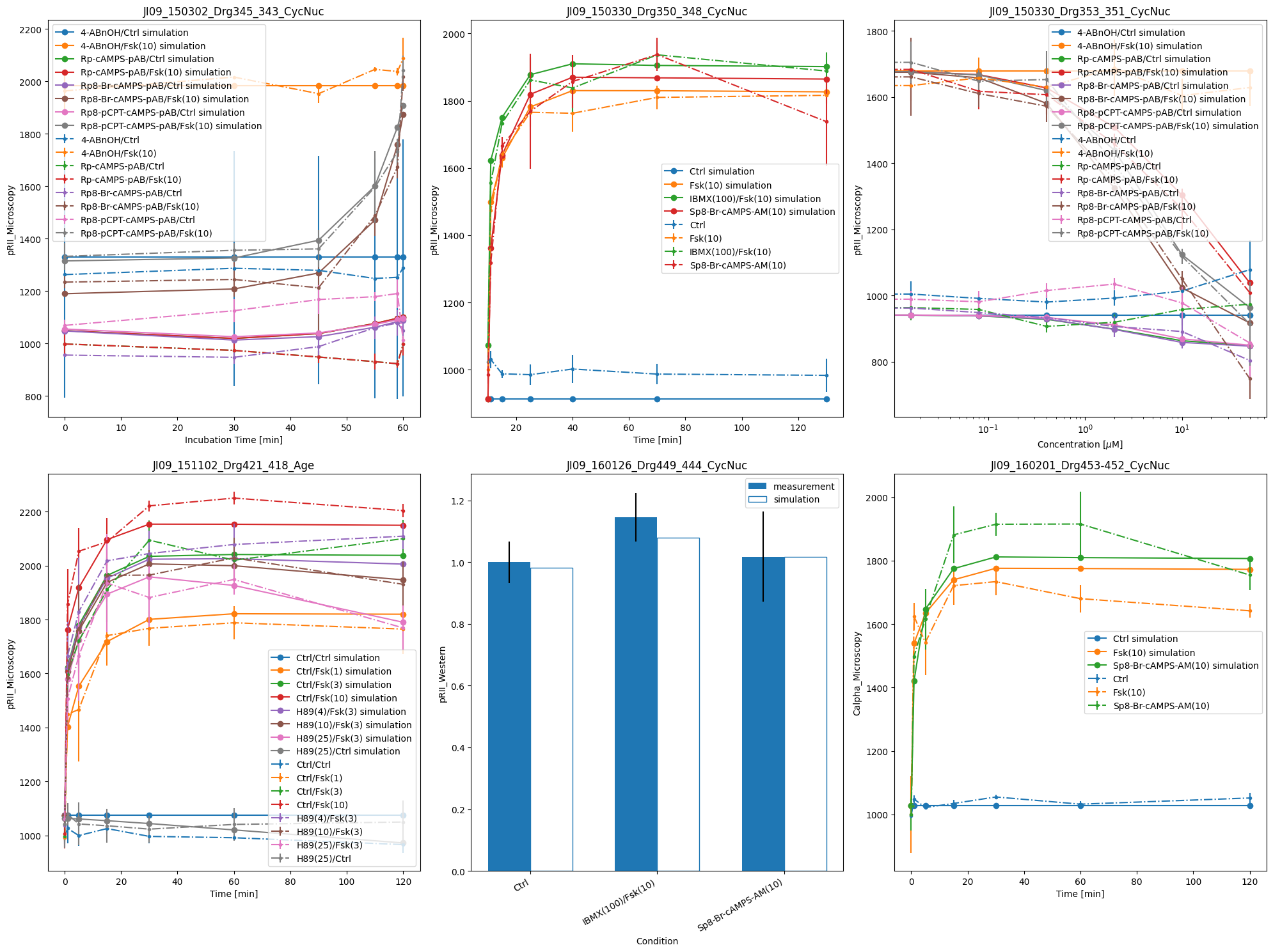
ax = plot_with_vis_spec(
    visualization_file_path,
    condition_file_path,
    data_file_path,
    simulation_file_path,
)

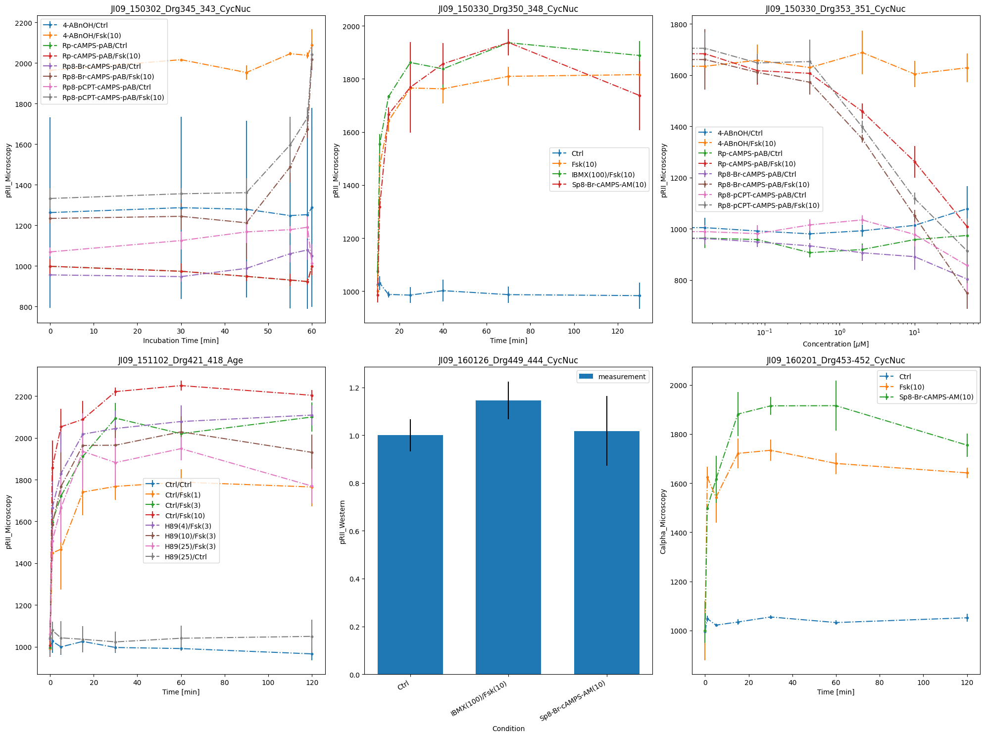
Now, we want to call the plotting routines without using the simulated data, only the visualization specification file.

ax_without_sim = plot_with_vis_spec(
    visualization_file_path, condition_file_path, data_file_path
)

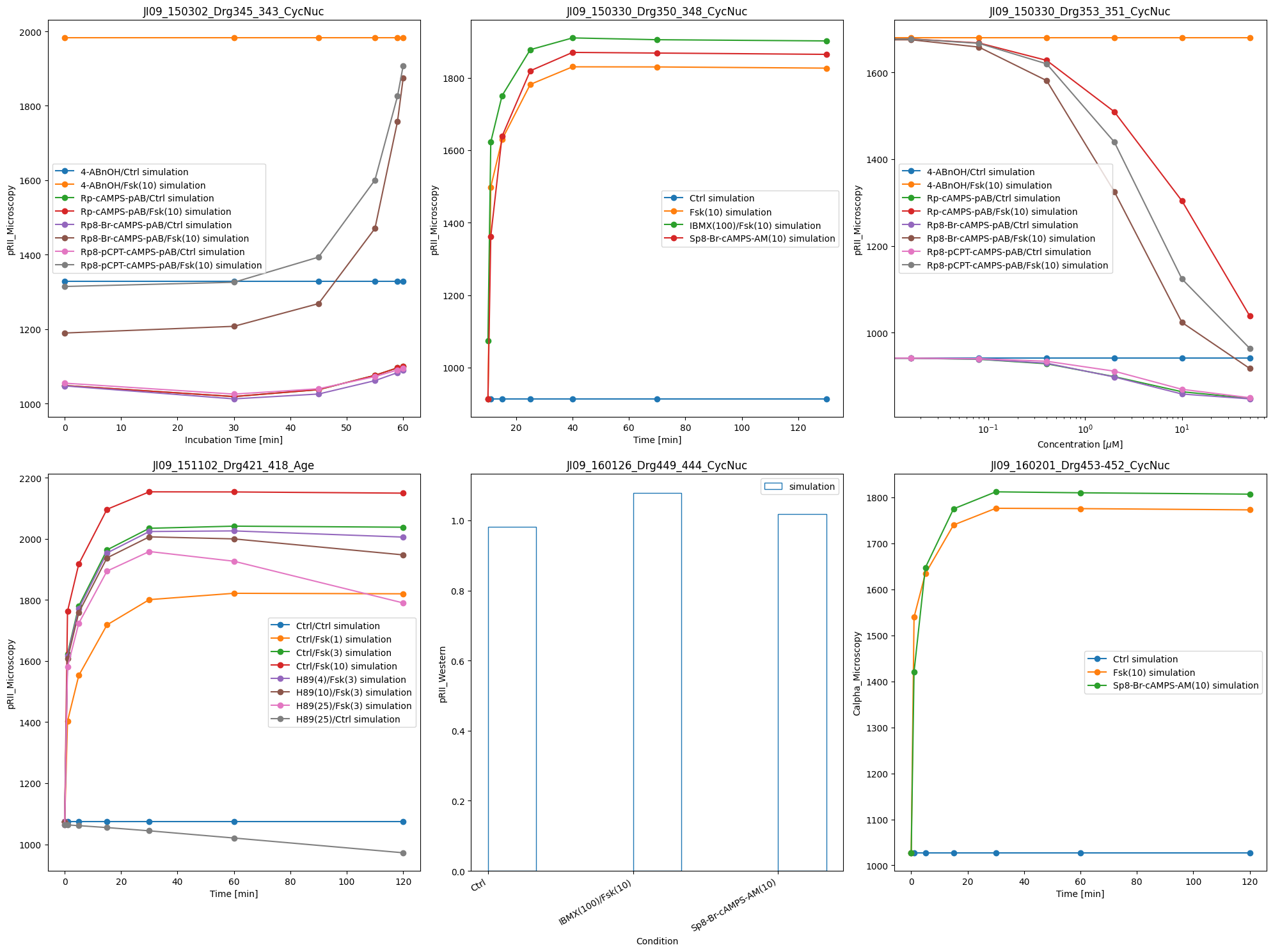
One can also plot only simulated data:

ax = plot_with_vis_spec(
    visualization_file_path,
    condition_file_path,
    simulations_df=simulation_file_path,
)

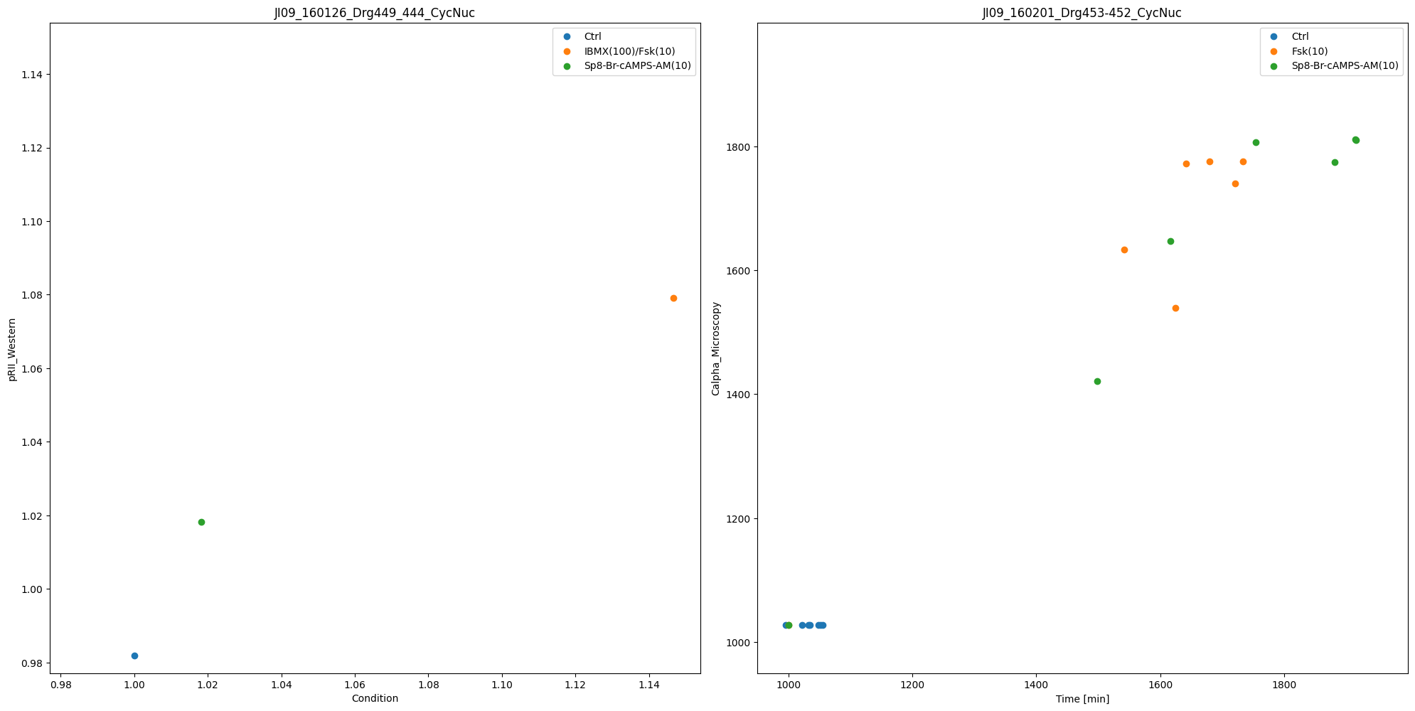
If both measurements and simulated data are available, they can be visualized using scatter plot:

visualization_file_scatterplots = (
    folder + "Isensee_visualizationSpecification_scatterplot.tsv"
)
ax = plot_with_vis_spec(
    visualization_file_scatterplots,
    condition_file_path,
    data_file_path,
    simulation_file_path,
)

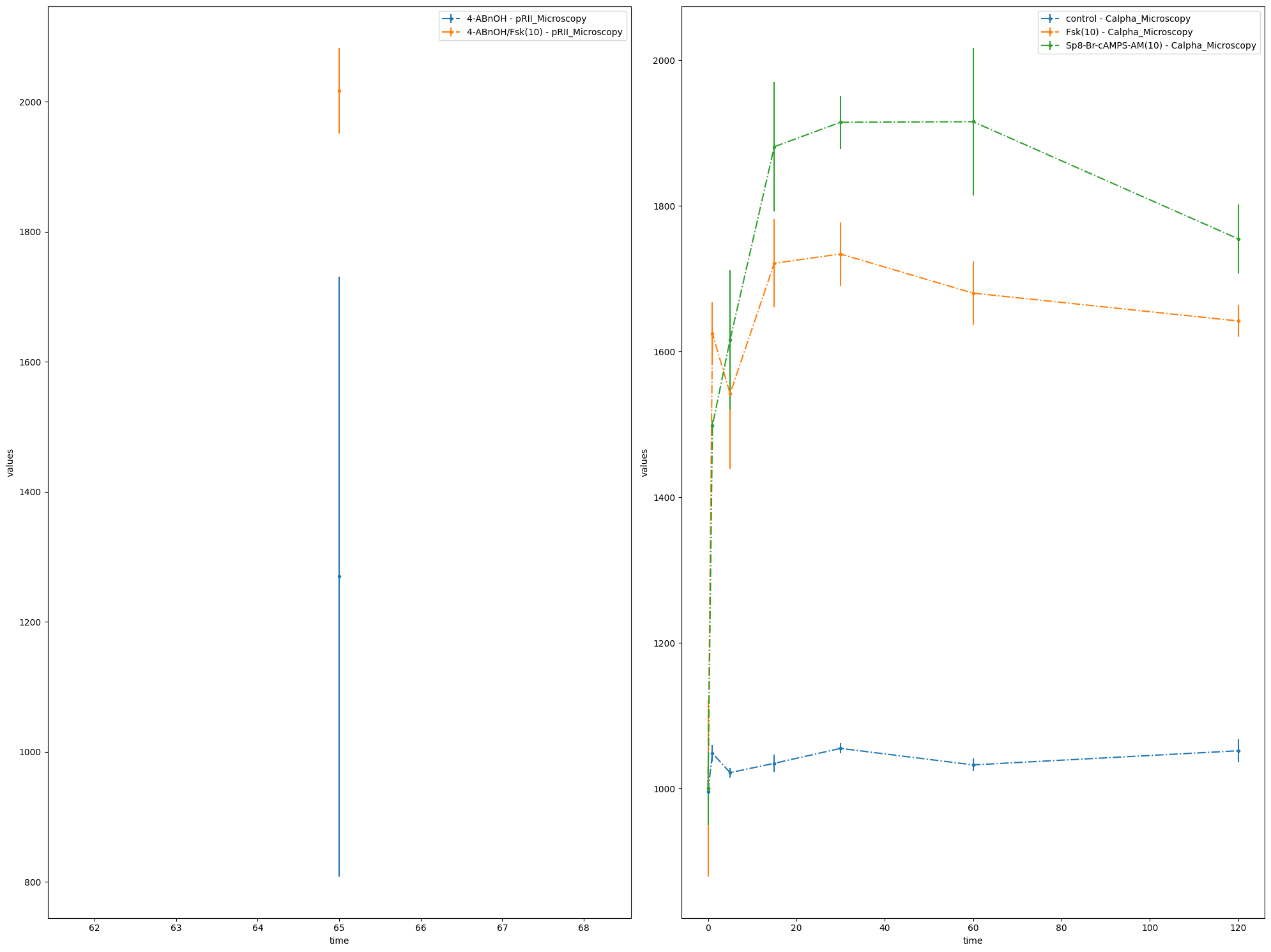
We can also call the plotting routine without the visualization specification file, but by passing a list of lists as dataset_id_list. Each sublist corresponds to a plot, and contains the datasetIds which should be plotted. In this simply structured plotting routine, the independent variable will always be time.

datasets = [
    [
        "JI09_150302_Drg345_343_CycNuc__4_ABnOH_and_ctrl",
        "JI09_150302_Drg345_343_CycNuc__4_ABnOH_and_Fsk",
    ],
    [
        "JI09_160201_Drg453-452_CycNuc__ctrl",
        "JI09_160201_Drg453-452_CycNuc__Fsk",
        "JI09_160201_Drg453-452_CycNuc__Sp8_Br_cAMPS_AM",
    ],
]
ax_without_sim = plot_without_vis_spec(
    condition_file_path, datasets, "dataset", data_file_path
)

Let’s look more closely at the plotting routines, if no visualization specification file is provided. If such a file is missing, PEtab needs to know how to group the data points. For this, three options can be used:

• dataset_id_list

• sim_cond_id_lis

• observable_id_list

Each of them is a list of lists. Again, each sublist is a plot and its content are either simulation condition IDs or observable IDs or the dataset IDs.

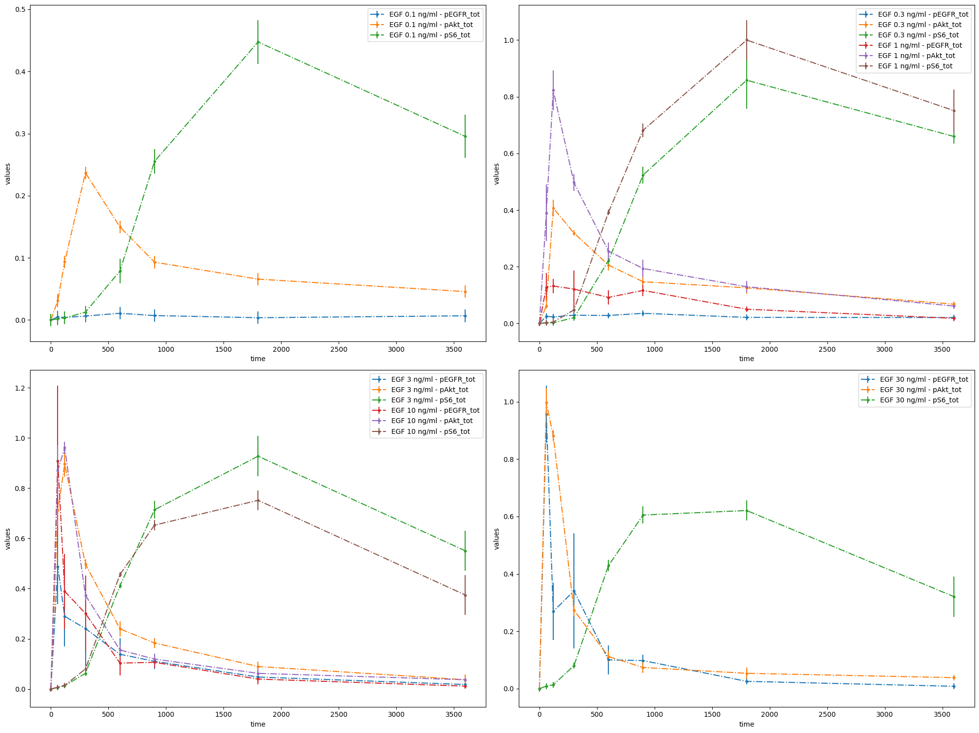
We want to illustrate this functionality by using a simpler example, a model published in 2010 by Fujita et al.

data_file_Fujita = "example_Fujita/Fujita_measurementData.tsv"
condition_file_Fujita = "example_Fujita/Fujita_experimentalCondition.tsv"

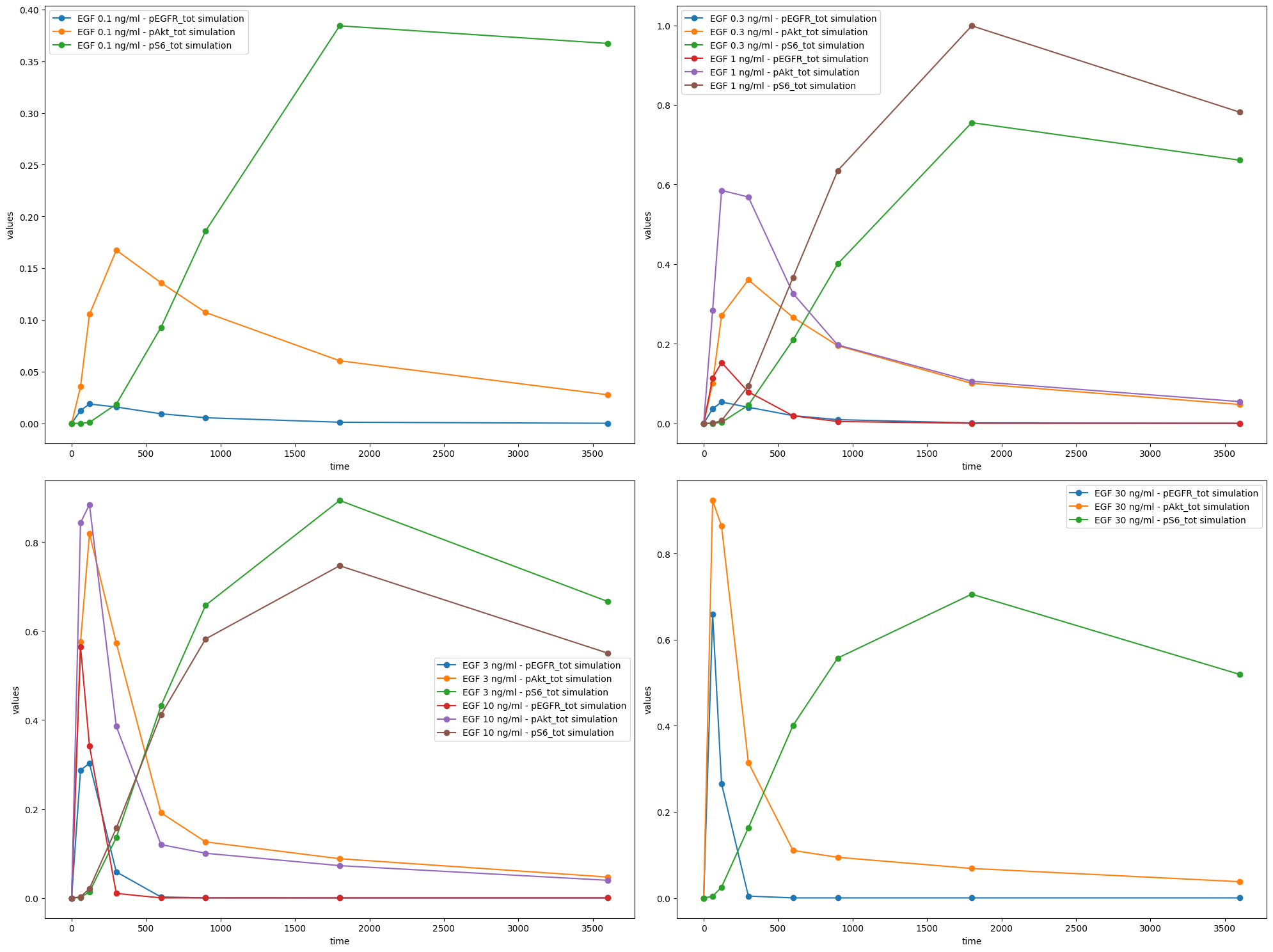
# Plot 4 axes objects, plotting
# - in the first window  all observables of the simulation condition 'model1_data1'
# - in the second window all observables of the simulation conditions 'model1_data2', 'model1_data3'
# - in the third window  all observables of the simulation conditions 'model1_data4', 'model1_data5'
# - in the fourth window all observables of the simulation condition 'model1_data6'

sim_cond_id_list = [
    ["model1_data1"],
    ["model1_data2", "model1_data3"],
    ["model1_data4", "model1_data5"],
    ["model1_data6"],
]

ax = plot_without_vis_spec(
    condition_file_Fujita,
    sim_cond_id_list,
    "simulation",
    data_file_Fujita,
    plotted_noise="provided",
)

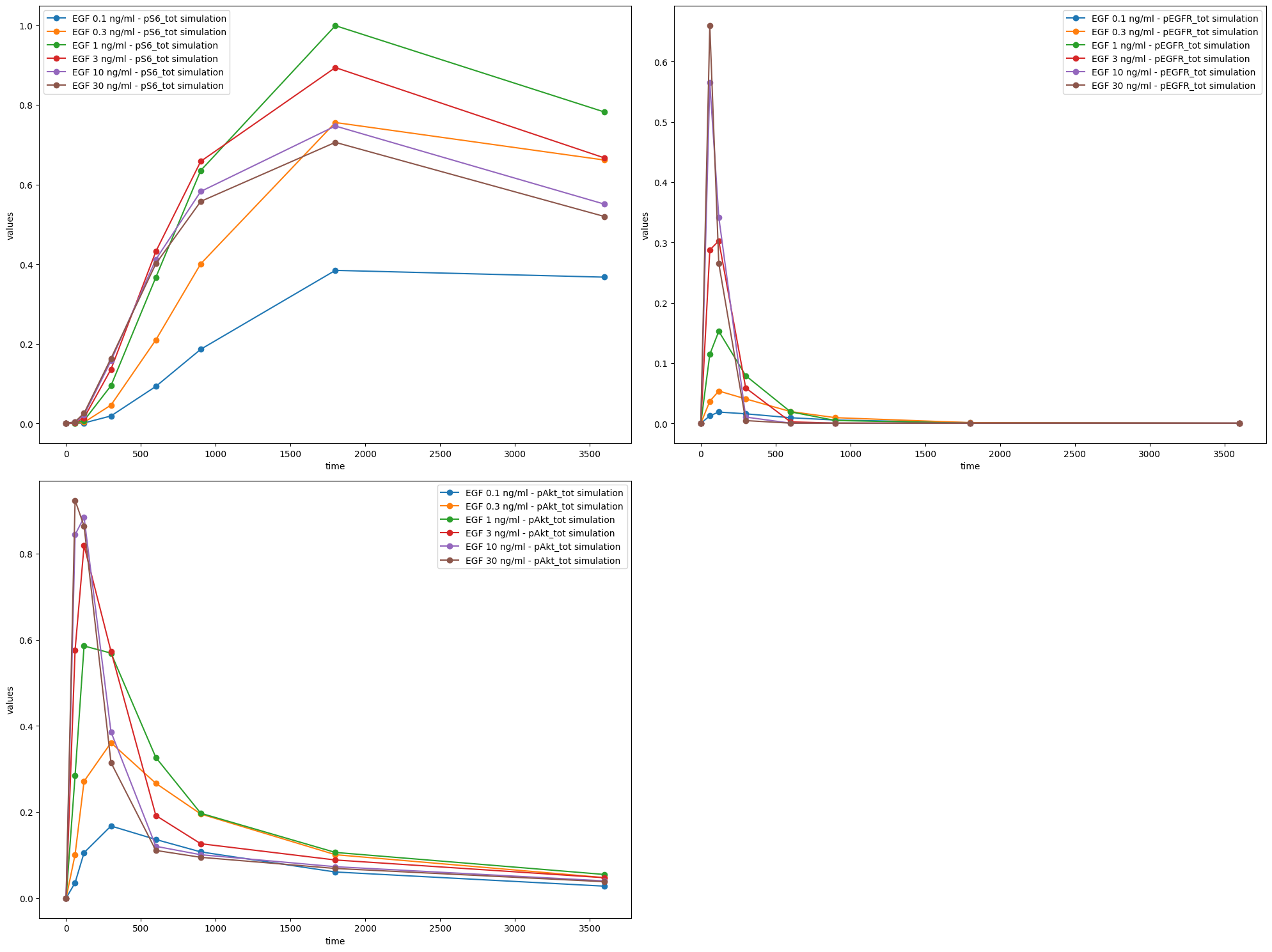
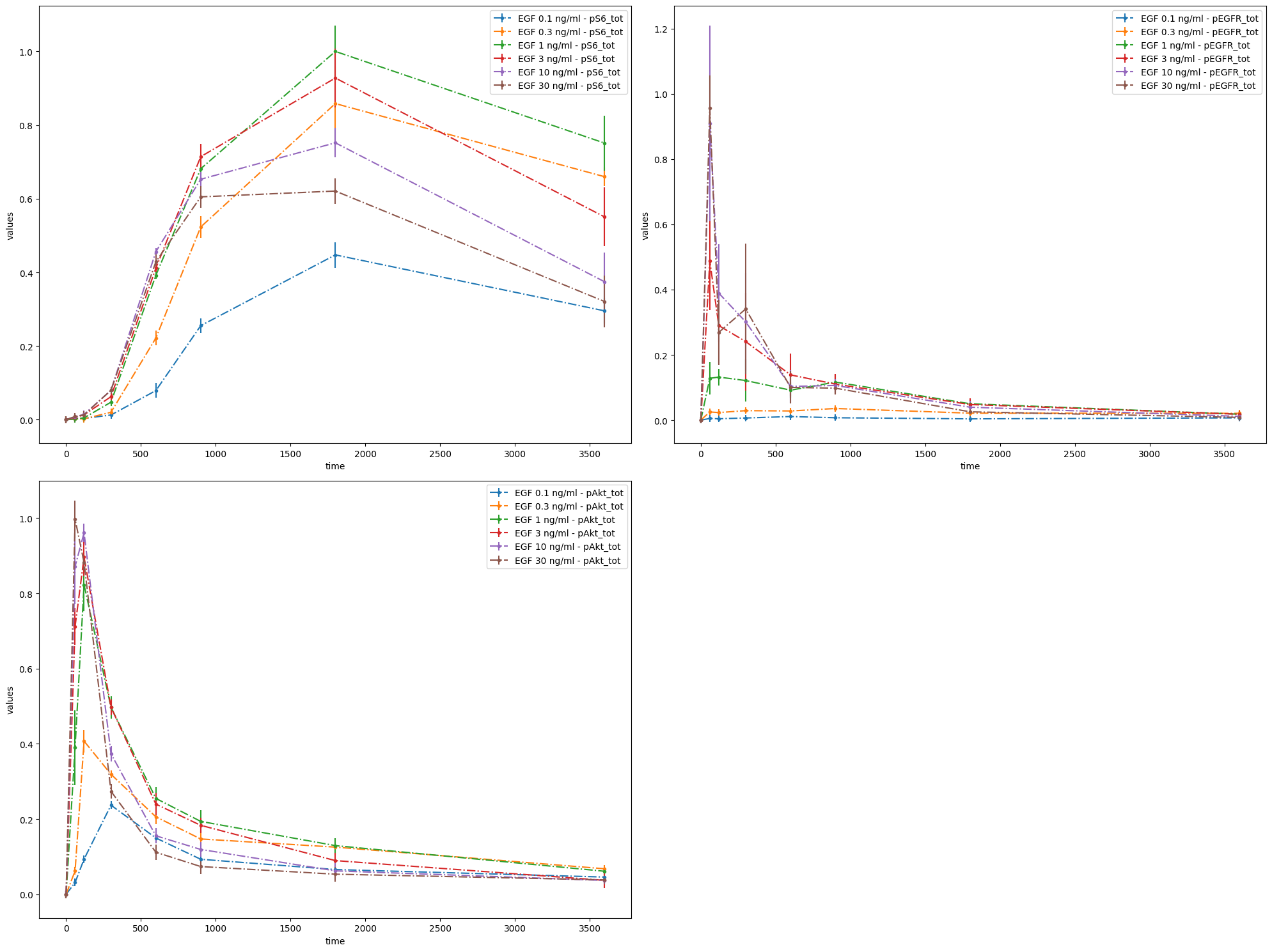
# Plot 3 axes objects, plotting
# - in the first window  the observable 'pS6_tot' for all simulation conditions
# - in the second window the observable 'pEGFR_tot' for all simulation conditions
# - in the third window  the observable 'pAkt_tot' for all simulation conditions

observable_id_list = [["pS6_tot"], ["pEGFR_tot"], ["pAkt_tot"]]


ax = plot_without_vis_spec(
    condition_file_Fujita,
    observable_id_list,
    "observable",
    data_file_Fujita,
    plotted_noise="provided",
)

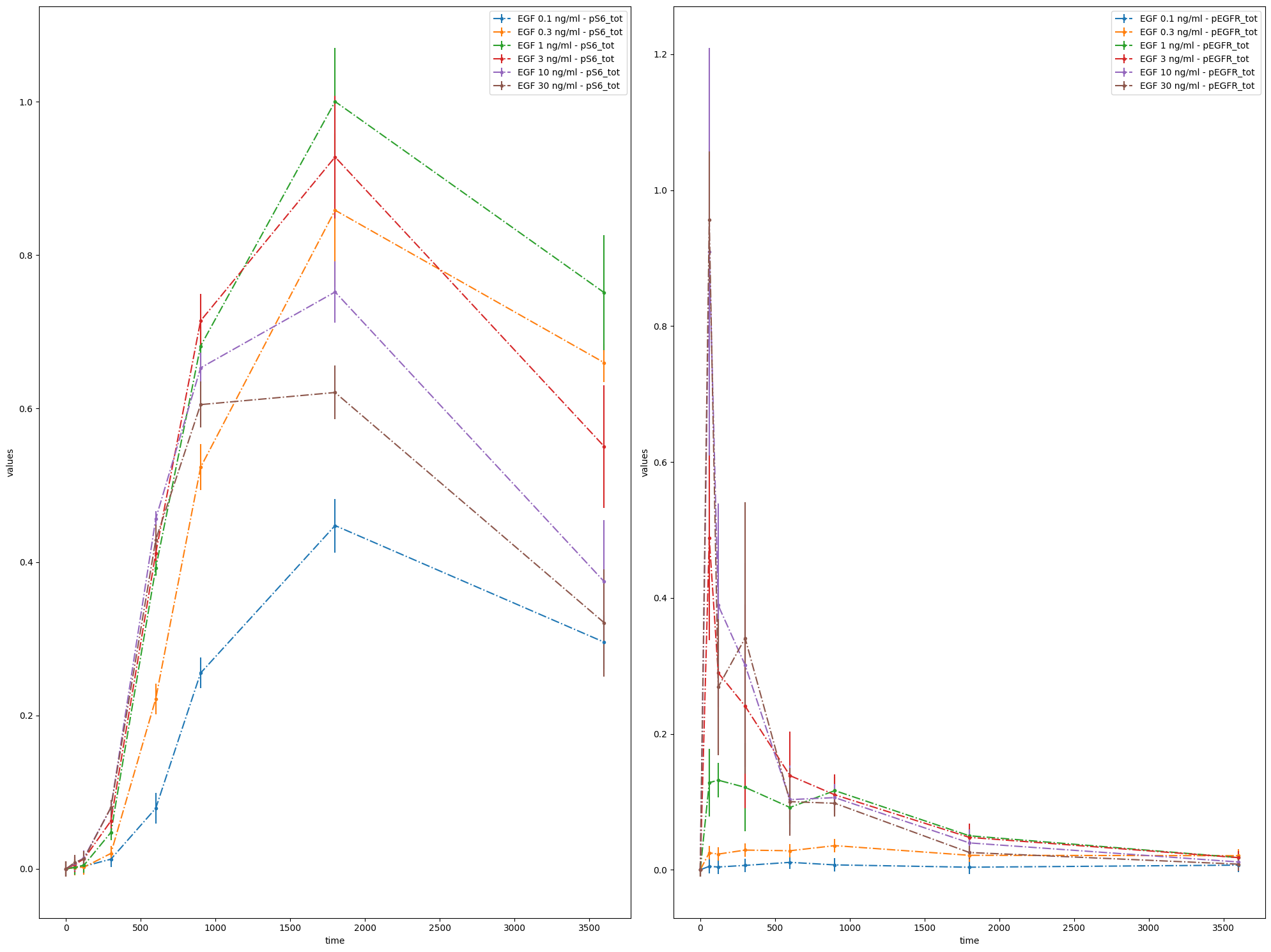
# Plot 2 axes objects, plotting
# - in the first window  the observable 'pS6_tot' for all simulation conditions
# - in the second window the observable 'pEGFR_tot' for all simulation conditions
# - in the third window  the observable 'pAkt_tot' for all simulation conditions
# while using the noise values which are saved in the PEtab files

observable_id_list = [["pS6_tot"], ["pEGFR_tot"]]


ax = plot_without_vis_spec(
    condition_file_Fujita,
    observable_id_list,
    "observable",
    data_file_Fujita,
    plotted_noise="provided",
)

Plot only simulations

simu_file_Fujita = "example_Fujita/Fujita_simulatedData.tsv"

sim_cond_id_list = [
    ["model1_data1"],
    ["model1_data2", "model1_data3"],
    ["model1_data4", "model1_data5"],
    ["model1_data6"],
]

ax = plot_without_vis_spec(
    condition_file_Fujita,
    sim_cond_id_list,
    "simulation",
    simulations_df=simu_file_Fujita,
    plotted_noise="provided",
)

observable_id_list = [["pS6_tot"], ["pEGFR_tot"], ["pAkt_tot"]]

ax = plot_without_vis_spec(
    condition_file_Fujita,
    observable_id_list,
    "observable",
    simulations_df=simu_file_Fujita,
    plotted_noise="provided",
)